This tutorial introduces the SGL language as well as usage of the rsgl package.
Setup
For use with the examples in this tutorial, we will create an
in-memory DuckDB database and load it
with two tables, cars and trees.
library(rsgl)
#>
#> Attaching package: 'rsgl'
#> The following objects are masked from 'package:datasets':
#>
#>     cars, trees
library(duckdb)
#> Loading required package: DBI

con <- dbConnect(duckdb())
#> duckdb is keeping downloaded extensions in a temporary directory:
#> ℹ /tmp/Rtmp4Qcx7h/duckdb/extensions
#> This is removed when the R session ends, so extensions are re-downloaded each session.
#> ℹ To keep them, point `options(duckdb.extension_directory =)` or the `DUCKDB_EXTENSION_DIRECTORY` environment variable at a permanent path.
dbWriteTable(con, "cars", cars)
dbWriteTable(con, "trees", trees)
Let’s query each to view a sample of data:
dbGetQuery(con, "
  select *
  from cars
  limit 5
")
#>   car_id horsepower miles_per_gallon origin year
#> 1      1        130               18    USA 1970
#> 2      2        165               15    USA 1970
#> 3      3        150               18    USA 1970
#> 4      4        150               16    USA 1970
#> 5      5        140               17    USA 1970
dbGetQuery(con, "
  select *
  from trees
  limit 5
")
#>   tree_id  age circumference
#> 1       1  118            30
#> 2       1  484            58
#> 3       1  664            87
#> 4       1 1004           115
#> 5       1 1231           120
dbGetPlot
The primary interface to rsgl is the dbGetPlot function,
which takes a DBI database
connection and a SGL statement and returns the corresponding plot.
Although the examples in this tutorial use a connection to a DuckDB
database, dbGetPlot will accept any DBI connection.
The SGL Language
The From Clause
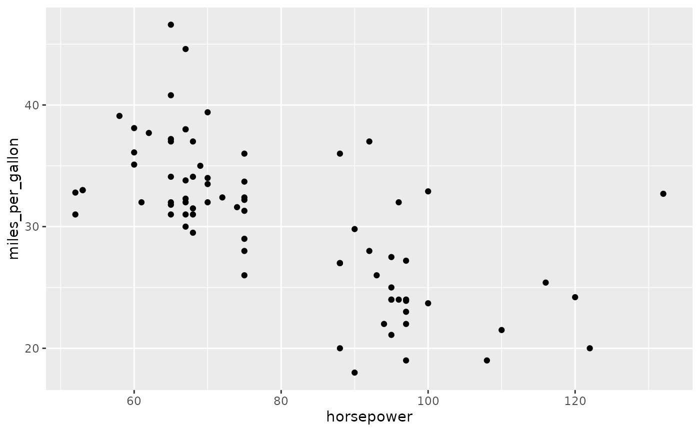
The from keyword precedes a data source specification,
which is often the name of a table in the database. Here, we specify the
cars table as the data source.
dbGetPlot(con, "
  visualize
    horsepower as x,
    miles_per_gallon as y
  from cars
  using points
")
This is similar in usage to the from keyword in SQL,
except that only a single data source is allowed (i.e., a
comma-separated list of table names is not valid). If data from multiple
sources or pre-processing of data is necessary, then a SQL subquery can
be provided:
dbGetPlot(con, "
  visualize
    horsepower as x,
    miles_per_gallon as y
  from (
    select *
    from cars
    where origin = 'Japan'
  )
  using points
")
The Using Clause
The using keyword precedes the name of the geometric
object(s) that will represent the data. Following ggplot2 terminology,
these geometric objects are referred to as geoms. Our previous examples
demonstrated representing data with point geoms.
The Visualize Clause
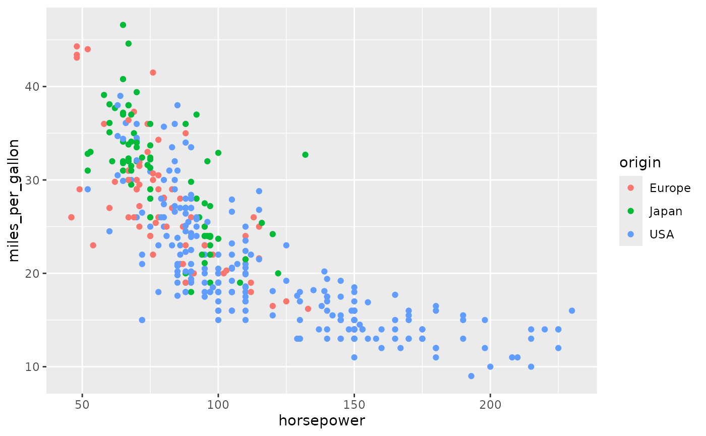
The visualize keyword precedes the aesthetic-to-column
mapping, which maps perceivable traits of the geoms to data source
columns. Our prior examples mapped the x and y
positions of the point geoms to data source columns. However, aesthetics
may be non-positional, as shown below. The visualize
keyword most closely resembles the select keyword within
SQL.
dbGetPlot(con, "
  visualize
    horsepower as x,
    miles_per_gallon as y,
    origin as color
  from cars
  using points
")
In addition to mapping aesthetics to columns, aesthetics can be mapped to expressions that include transformations and aggregations.
Column-Level Transformations and Aggregations
SGL supports column-level transformations and aggregations, as shown
below where a binning transformation is combined with a count
aggregation to produce a histogram on miles_per_gallon.
dbGetPlot(con, "
  visualize
    bin(miles_per_gallon) as x,
    count(*) as y
  from cars
  group by
    bin(miles_per_gallon)
  using bars
")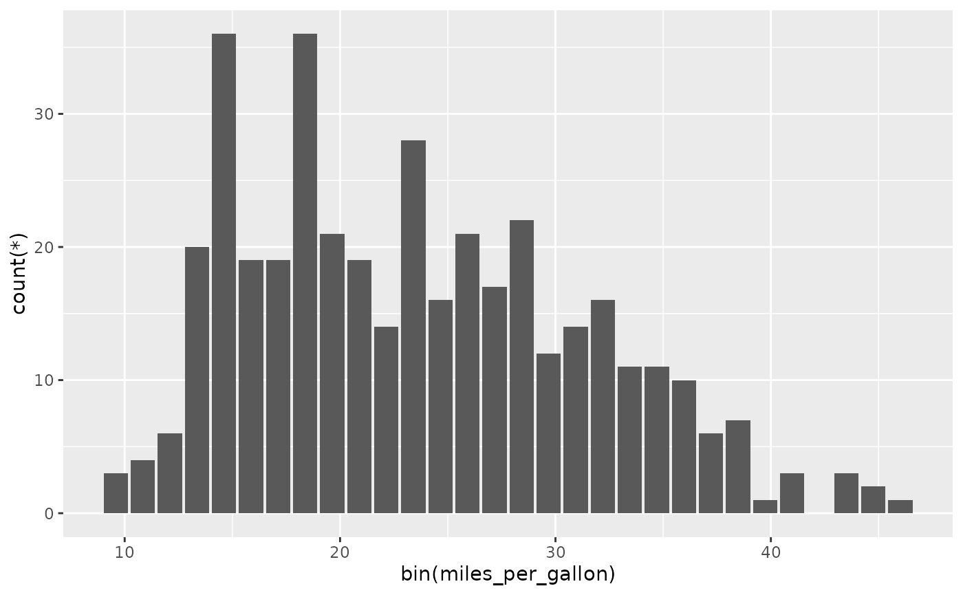
Here we see that, similarly to SQL, SGL has a group by
clause where aggregation groupings are specified.
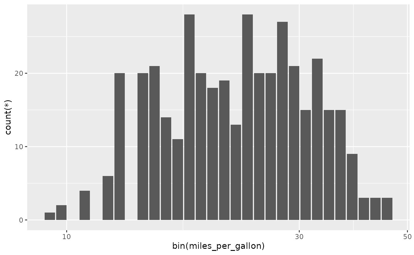
Although SQL itself supports column-level transformation, grouping, and aggregation, it is desirable for SGL to provide additional support for these operations. Statistical graphics often require operations such as binning that are not natively supported by SQL. Additionally, SGL’s column-level transformations and aggregations are performed after scaling, which cannot easily be replicated using SQL. Below is an example of this feature, where binning and counting are applied after log scaling, resulting in a log-scaled histogram.
dbGetPlot(con, "
  visualize
    bin(miles_per_gallon) as x,
    count(*) as y
  from cars
  group by
    bin(miles_per_gallon)
  using bars
  scale by
    log(x)
")
The Collect By Clause
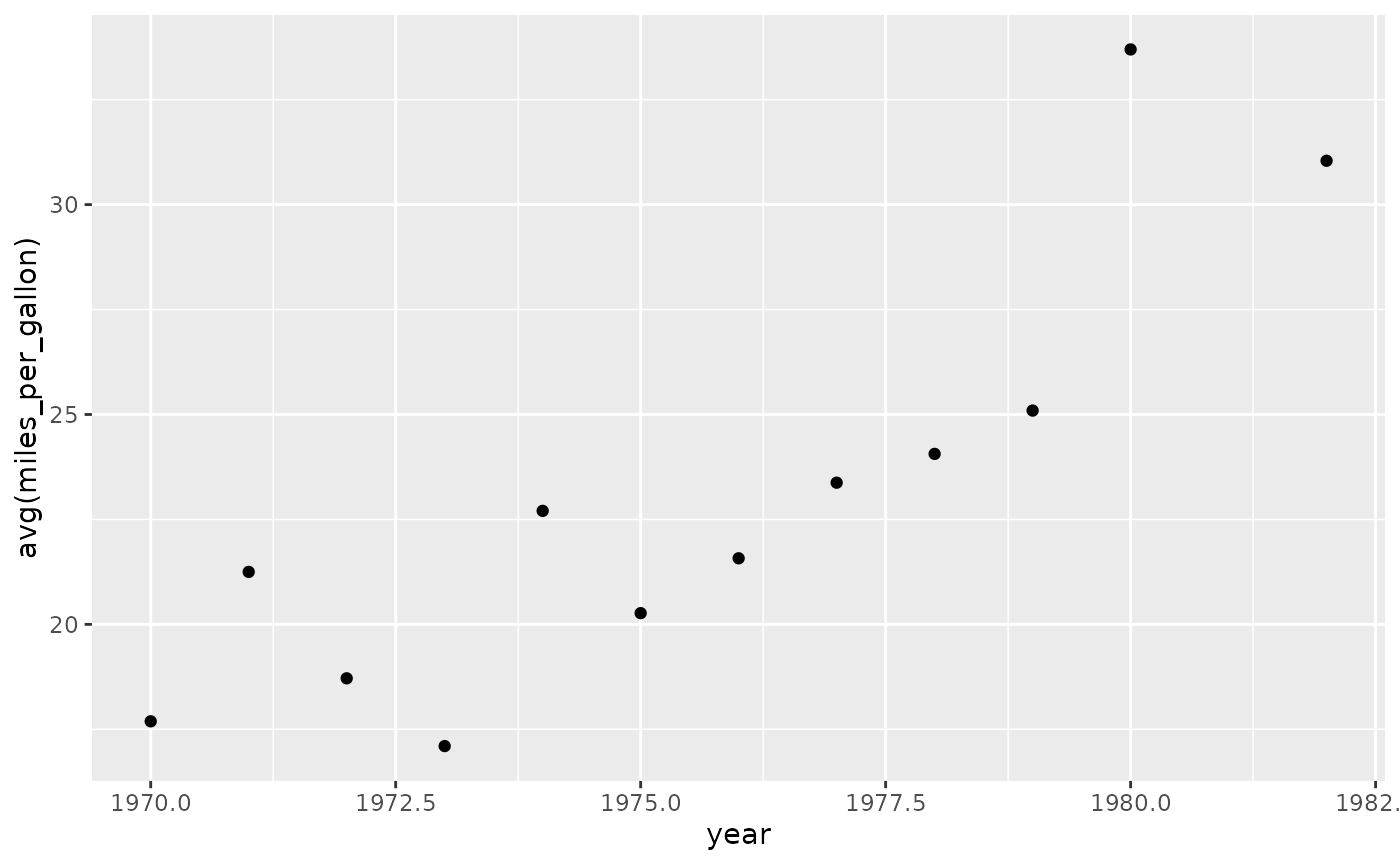
In SGL, a geom is classified as individual if it represents each record (after transformation and aggregation) by a distinct geometric object. Alternatively, a geom is classified as collective if it represents multiple records by one geometric object. For example, points and lines are individual and collective geoms, respectively, as shown below where the same data is represented using each.
dbGetPlot(con, "
  visualize
    year as x,
    avg(miles_per_gallon) as y
  from cars
  group by
    year
  using points
")
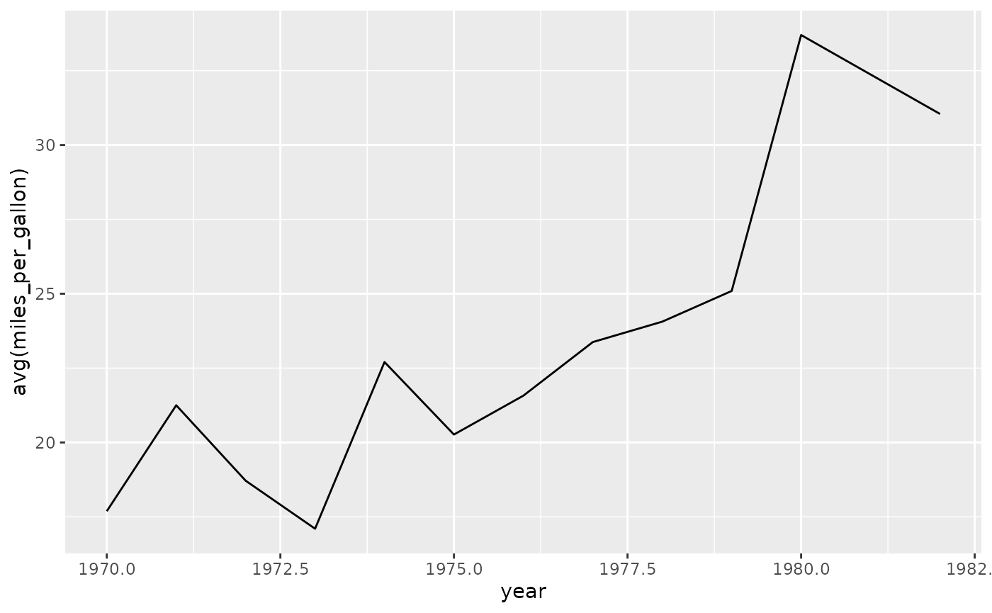
dbGetPlot(con, "
  visualize
    year as x,
    avg(miles_per_gallon) as y
  from cars
  group by
    year
  using line
")
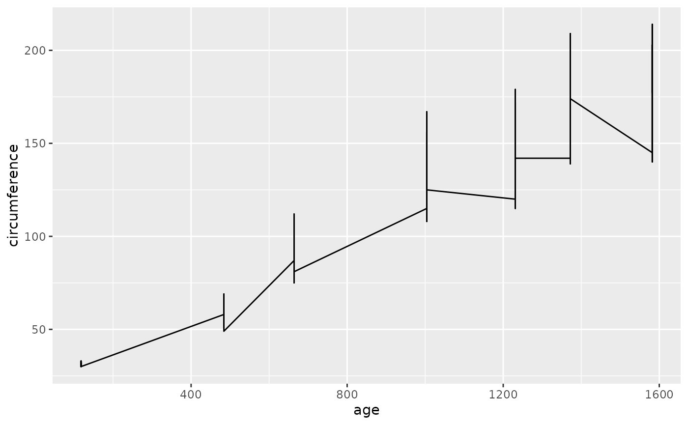
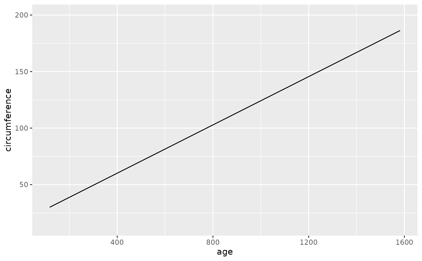
For collective geoms, the collection of records to represent by each
object is determined automatically using reasonable defaults. This
behavior can be overridden by providing explicit collections in the
collect by clause. The collect by clause is
similar to the group by clause, except that rather than
defining groups to aggregate by, the collect by clause
defines collections of records to be represented by one object. Below we
see an example where the default collection is not ideal, followed by a
preferrable explicit collection.
dbGetPlot(con, "
  visualize
    age as x,
    circumference as y
  from trees
  using line
")
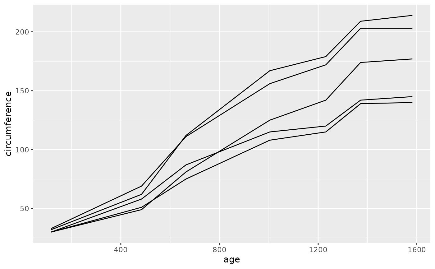
dbGetPlot(con, "
  visualize
    age as x,
    circumference as y
  from trees
  collect by
    tree_id
  using lines
")
Geom Qualifiers
Geom qualifiers modify how geoms positionally represent data, and are
specified as keywords that precede geom names within the
using clause. Geom qualifiers can largely be classified
into two groups, statistical qualifiers and collision qualifiers.
Statistical qualifiers modify the positional representation via
statistical transformation, such as linear regression:
dbGetPlot(con, "
  visualize
    age as x,
    circumference as y
  from trees
  using regression line
")
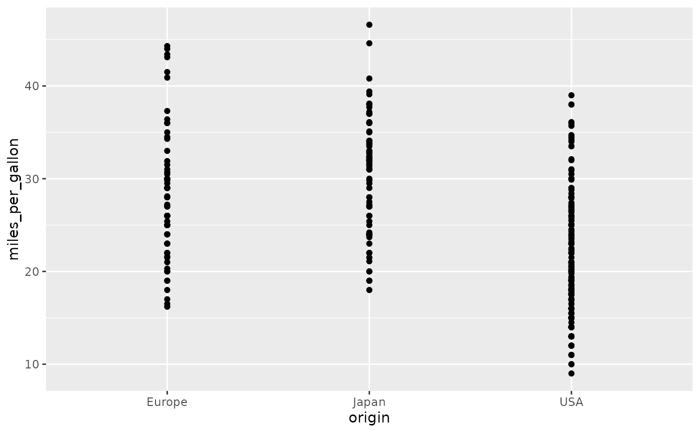
Collision qualifiers specify positional adjustments that are relevant
to overlapping objects. Below we see an example of using the
jittered qualifier to add a small amount of random
variation so that overlapping points are discernible.
Without the jittered qualifier:
dbGetPlot(con, "
  visualize
    origin as x,
    miles_per_gallon as y
  from cars
  using points
")
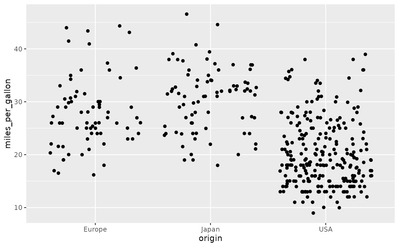
With the jittered qualifier:
dbGetPlot(con, "
  visualize
    origin as x,
    miles_per_gallon as y
  from cars
  using jittered points
")
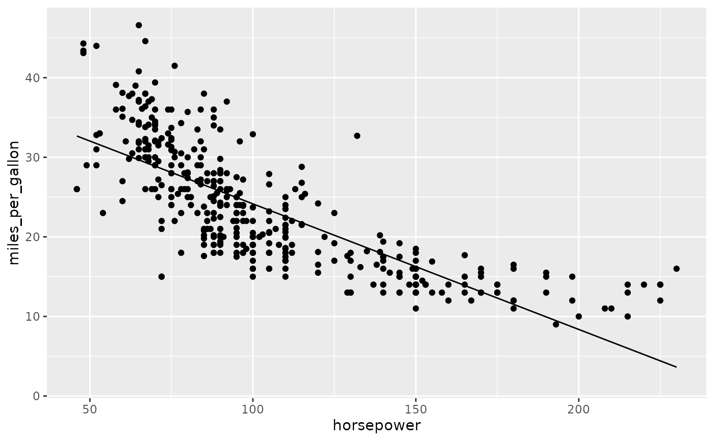
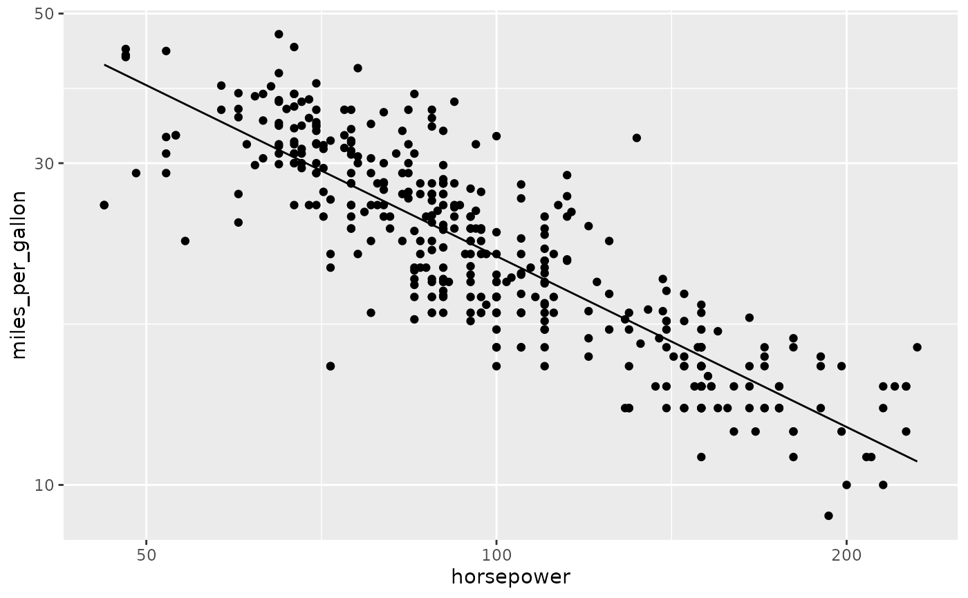
The Layer Operator
The graphics in previous sections contain a single layer of geometric
objects. However, it is common to use multiple layers of objects to
represent data in a single graphic. In SGL, multiple layers can be
combined using the layer operator. For example, we can
layer a regression line on a scatterplot:
dbGetPlot(con, "
  visualize
    horsepower as x,
    miles_per_gallon as y
  from cars
  using points

  layer

  visualize
    horsepower as x,
    miles_per_gallon as y
  from cars
  using regression line
")
Layers often share a data source and aesthetic mapping. To reduce
verbosity in these cases, the layer operator can be applied
directly to geom expressions:
dbGetPlot(con, "
  visualize
    horsepower as x,
    miles_per_gallon as y
  from cars
  using (
    points
    layer
    regression line
  )
")
Layers may have different data sources and aesthetic mappings. However, a graphic has a single scale for each aesthetic, regardless of the number of layers. As a result, a given aesthetic must be mapped to consistent type across all layers where it is present, e.g. an aesthetic cannot be mapped to a numerical type in one layer and a categorical type in another.
The Scale By Clause
Each mapped aesthetic has a scale that determines how data values are
mapped to the corresponding visual property. Scales are determined
implicitly by default, but can be explicitly specified within the
scale by clause. Below we specify a log scale
for the x and y aesthetics, overriding the
default linear scaling for numerical mappings:
dbGetPlot(con, "
  visualize
    horsepower as x,
    miles_per_gallon as y
  from cars
  using (
    points
    layer
    regression line
  )
  scale by
    log(x), log(y)
")
Scaling is performed prior to column-level transformations and aggregations. Additionally, scaling is performed prior to any positional modifications specified by geom qualifiers, e.g., the regression calculation above is performed after log-scaling the x and y aesthetics.
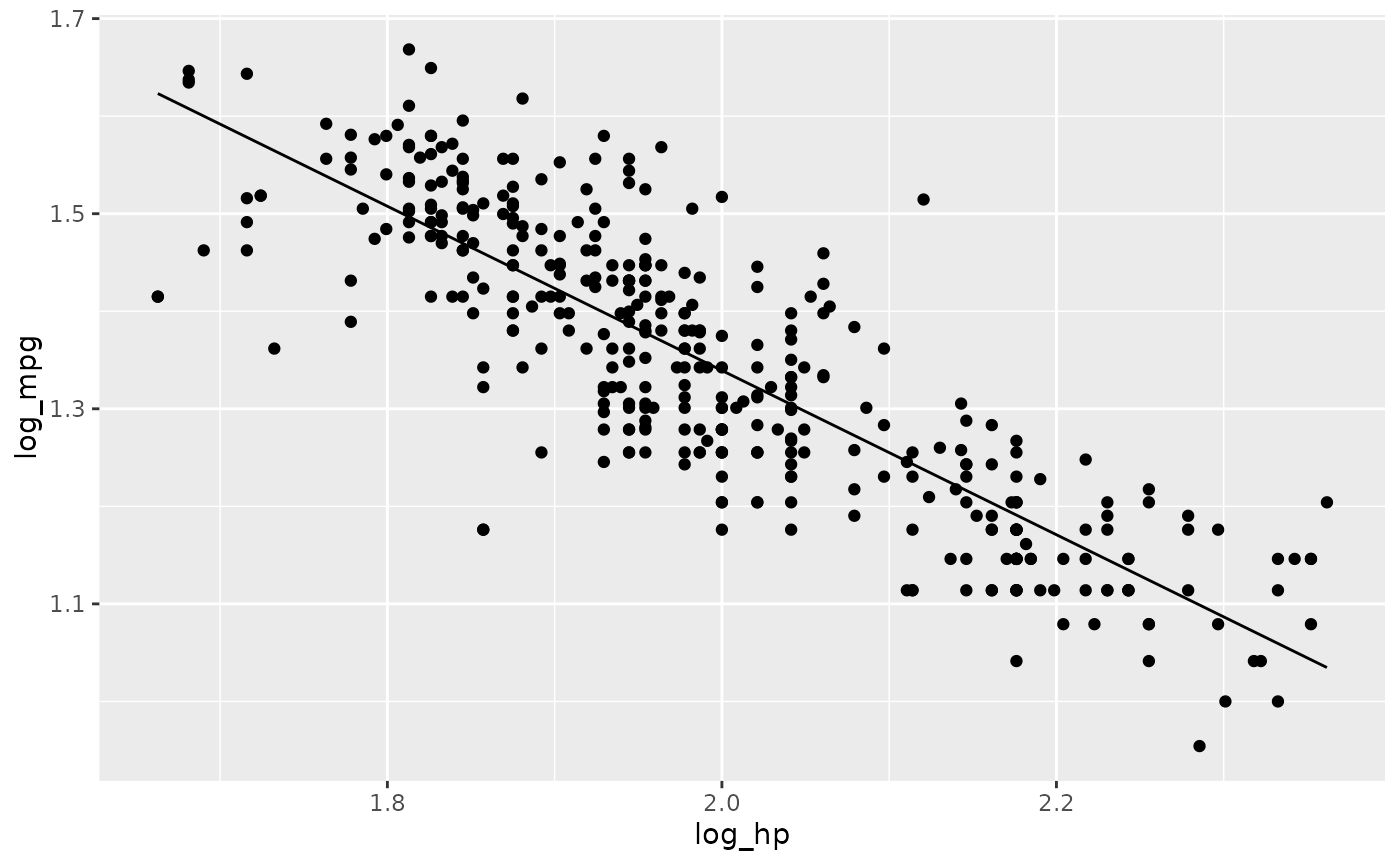
Scaling functions such as log are applied to aesthetic
names rather than column names as these are modifications to aesthetic
scales rather than actual data values. This distinction is demonstrated
below, where a log function is instead applied to actual
data values in a SQL subquery:
dbGetPlot(con, "
  visualize
    log_hp as x,
    log_mpg as y
  from (
    select
      log(horsepower) as log_hp,
      log(miles_per_gallon) as log_mpg
    from cars
  )
  using (
    points
    layer
    regression line
  )
")
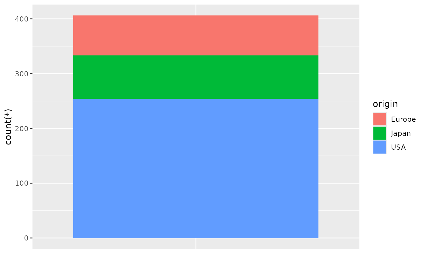
Coordinate Systems
The graphics in prior examples use Cartesian coordinates, but
alternative coordinate systems are valid. In SGL, the coordinate system
is inferred from the positional aesthetics in the visualize
clause. For example, x and y aesthetics imply
Cartesian coordinates, whereas theta and r
imply polar coordinates.
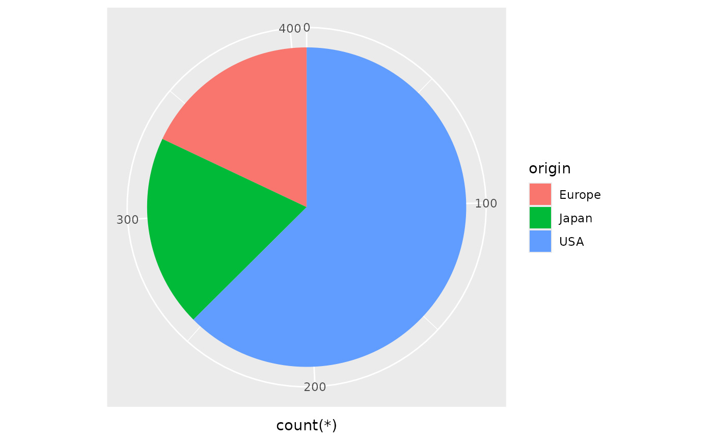
The examples below display the same information in Cartesian and polar coordinates. In the grammar of graphics (which SGL is based on), pie charts are stacked bar charts in a polar coordinate system. In SGL, the bar geom is stacked by default.
dbGetPlot(con, "
  visualize
    count(*) as y,
    origin as color
  from cars
  group by
    origin
  using bars
")
dbGetPlot(con, "
  visualize
    count(*) as theta,
    origin as color
  from cars
  group by
    origin
  using bars
")
Since a SGL statement may have multiple layers, it may also have
multiple visualize clauses, each with positional aesthetic
mappings. Since a graphic has a single coordinate system, the positional
aesthetics referenced across layers must be consistent, e.g. one layer
cannot reference x and y aesthetics while
another references theta and r.
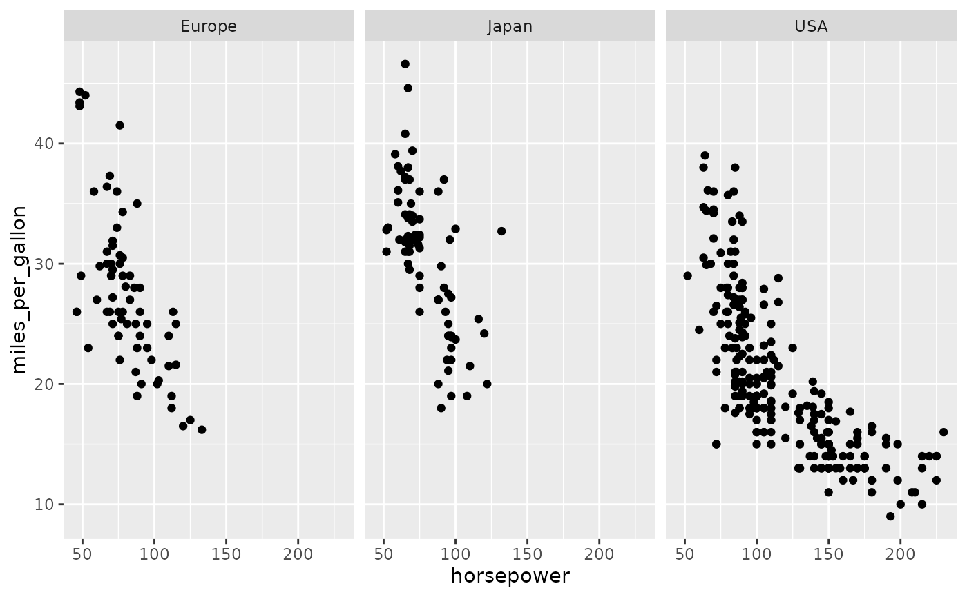
The Facet By Clause
Faceting generates small multiples where each panel represents a
different partition of the source data. Partitioning is determined by
the unique values for expressions specified in the facet by
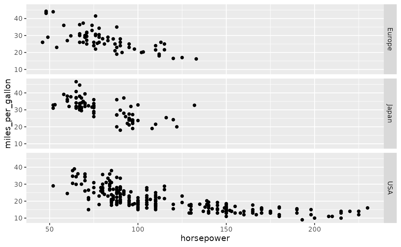
clause. Faceting by a single expression generates horizontal panels by
default, but this can be modified with an orientation keyword:
dbGetPlot(con, "
  visualize
    horsepower as x,
    miles_per_gallon as y
  from cars
  using points
  facet by
    origin
")
dbGetPlot(con, "
  visualize
    horsepower as x,
    miles_per_gallon as y
  from cars
  using points
  facet by
    origin vertically
")
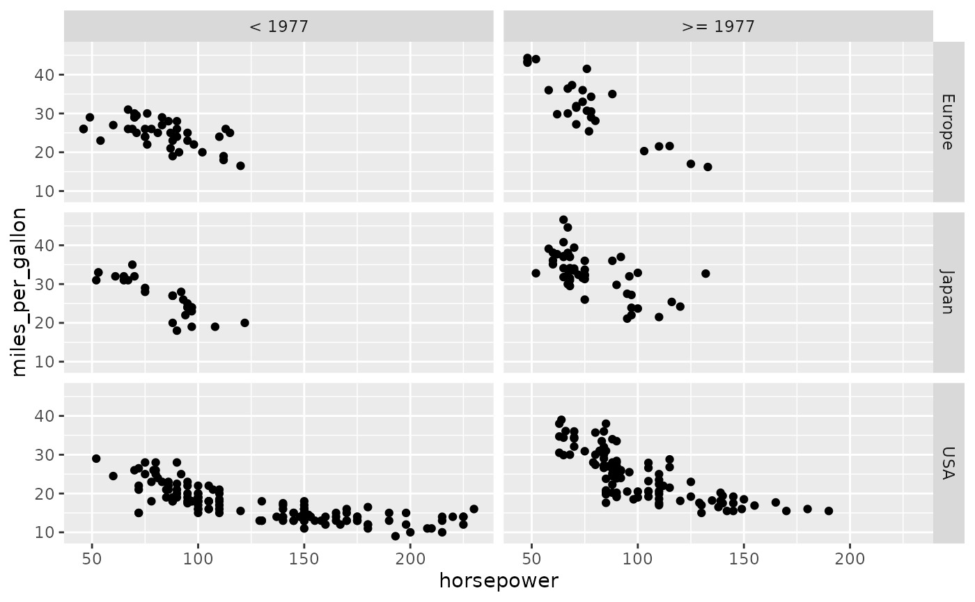
Two facet expressions may be specified, in which case one expression is represented horizontally while the other is represented vertically:
dbGetPlot(con, "
  visualize
    horsepower as x,
    miles_per_gallon as y
  from (
    select
      *,
      case
        when year < 1977
        then '< 1977'
        else '>= 1977'
      end as 'era'
    from cars
  )
  using points
  facet by
    era,
    origin
")
In SGL, facets are a graphic-level property, meaning that each SGL
statement has at most one facet by clause, and that each
layer is faceted accordingly.
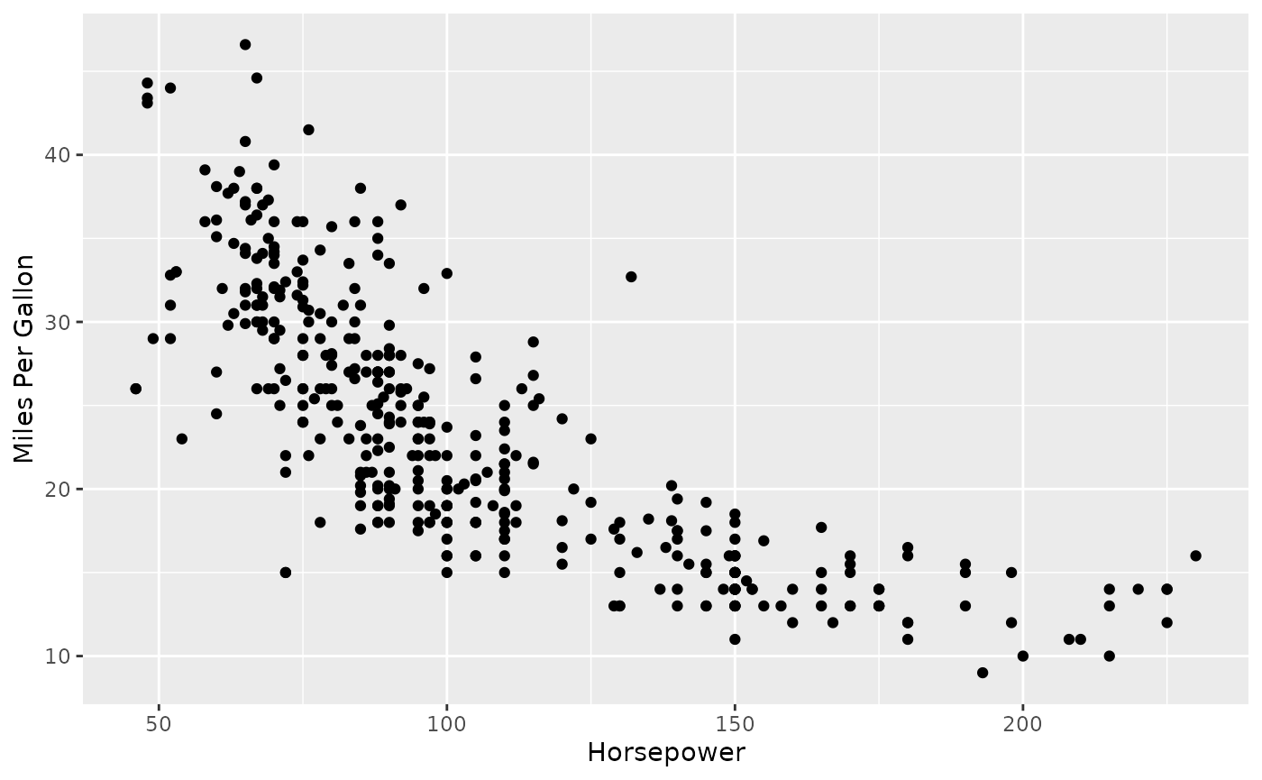
The Title Clause
Titles for aesthetic scales are automatically determined from
aesthetic mappings. However, this can be overridden by providing
explicit titles in the title clause:
dbGetPlot(con, "
  visualize
    horsepower as x,
    miles_per_gallon as y
  from cars
  using points
  title
    x as 'Horsepower',
    y as 'Miles Per Gallon'
")
Next steps
- Reference — details on the specific geoms, aesthetics, qualifiers, transformations, aggregations, and scales available in rsgl.
- Example gallery — a collection of plots generated with rsgl.
- SGL Paper — covers the language in greater depth, including SGL’s underlying grammar of graphics.